Whole Genome & Transcriptome Sequencing (WGTS) Reports

Djerba INI configuration

The config.ini file created in Set up a Djerba working directory is empty by default and some fields must be filled by the CGI staff. The INI can be edited either in the command line (using nano or vim) or using a text editor. An empty INI is shown below. Values shown as REQUIRED must be filled in by the CGI staff. The example file was generated for the WGTS assay. It is an illustrative example only; plugin parameters may change from time to time. The automatic setup in Set up a Djerba working directory will create a config.ini file with up-to-date parameters:

[core]

[input_params_helper]
assay = REQUIRED
donor = REQUIRED
oncotree_code = REQUIRED
primary_cancer = REQUIRED
project = REQUIRED
requisition_approved = REQUIRED
requisition_id = REQUIRED
sample_type = REQUIRED
site_of_biopsy = REQUIRED
study = REQUIRED

[wgts.cnv_purple]

[report_title]

[patient_info]

[expression_helper]

[provenance_helper]

[wgts.snv_indel]

[genomic_landscape]

[case_overview]

[fusion]

[sample]

[summary]

[supplement.body]

[gene_information_merger]

[treatment_options_merger]

The underlying INI syntax conforms to the Python ConfigParser module. Empty parameters do not require specification and can be left out of the .ini – section headers (denoted by square brackets) are used by Djerba to discover which plugins to load and therefore must be included even if all parameters are left blank.

Summary of INI parameters:

The parameters below are entered in the [input_params_helper] section of the INI file and the information is obtained either from one of two Data Sources: the Requisition (Req) system or Dimsum.

• Navigating the Requisition System

• Navigating Dimsum

INI parameter	Description	Data source
assay	One of WGTS, WGS, TAR, PWGS	Req system
donor	Donor LIMS ID, eg. PANX_1249	Dimsum
oncotree_code	OncoTree code, case-insensitive (eg. paad)	Req system
requisition_approved	Date of first requisition approval by Tissue Portal staff in yyyy-mm-dd format	Req system
project	name of the project in provenance	Dimsum
requisition_id	I.D. in requisition system	Req system
sample_type	Select submission type	Req system
primary_cancer	Select primary cancer type	Req system
site_of_biopsy	Site of biopsy/surgery	Req system
study	Name of study (acronym) in requisition system	Req system

Completed [core] and [input_params_helper] sections in the INI file:

[core]

[input_params_helper]
assay = WGTS
donor = PANX_1249
oncotree_code = paad
primary_cancer = Pancreatic Adenocarcinoma
project = PASS01
requisition_approved = 2021-03-29
requisition_id = PASS01UHN-115
sample_type = LCM
site_of_biopsy = Liver
study = PASS-01

For further details on the INI file, or how to troubleshoot when discovered parameters don’t fill automatically, see Djerba documentation.

Interim Report Generation

With the completed .ini, generate the interim report according to the following steps:

1. Login and setup the analysis environment on a Univa compute node, as described in Set up a Djerba working directory.

2. Run the djerba.py script using the INI file completed in Djerba INI configuration and the ‘report’ subdirectory created in Set up a Djerba working directory

   $ djerba.py report -i  my/path/config.ini -o /my/output/dir/ -p
   

Output filename is of the form ${TUMOUR_ID}+${version}.html in the report directory.

Review Tumour Quality

In the “Sample Information” section, review sample quality information for the tumour.

CGI staff are responsible for verification of two quality metrics - Callability and Estimated Cancer Cell Content. If a case does not pass either metric, it cannot continue with the assay and must be failed.

Callability

Callability is defined as the percentage of bases with at least 30X coverage in the tumour. Callability is calculated in pipeline and recorded in QC-ETL. This value is automatically retrieved by Djerba. Verify the value in the Djerba provisional report passes the necessary threshold (as defined in QM-024. Quality Control and Calibration Procedures🔒 SOP).

Note

If a sample’s callability falls below that threshold but qualifies under the “Callability Metric Override” outlined in QM-0024, the clinical report will still be generated and issued normally, without requiring a planned deviation. When signing off on analysis review, add a note to the QC report stating that the sample meets callability override metrics and that the report passes.

Estimate Cancer Cell Content

In the process of estimating cancer cell content, most software consider many ploidy/purity solutions. The CGI staff need to evaluate whether the best solution was chosen by the software. If the chosen cancer cell content is below the threshold in QM-024. Quality Control and Calibration Procedures🔒 SOP, a failed report should be generated (see Failed WGTS Report). Estimated Cancer Cell Content (Purity) must also be recorded in MISO by staff (Updating QCs)

Procedure

Investigate the PURPLE range and segment_QC plots to see whether the default solution is optimal.

Considerations:

• The default primary solution is typically preferred

• Prioritize solutions close to diploid (N=2); generally, lower ploidy solutions are preferred to higher ploidy. Ploidies ≥ 5N with low purities should be investigated with high skepticism.

• Compare cancer cell content to the VAF of driver mutations: while PURPLE does consider the VAF distribution in choosing a solution, known common mutations with LOH (such as TP53) are informative markers of the sample’s cancer cell content. The VAF of variants with LOH often reflects the tumor purity.

• Common signals in the VAF distribution that something is wrong:

Abnormality	Potential Cause	Action
Skewed distribution towards 0% VAF	Low purity	Confirm purity > 30%
Excessive VAFs at 50% and 100%	Germline Contamination	Check for swap

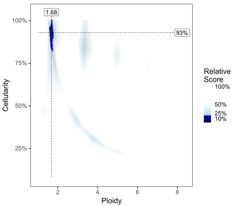
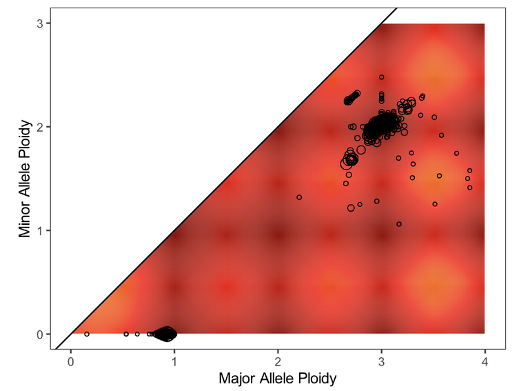
To review solutions, open the file purple.range.png in the working directory. The contour plot shows the relative likelihood for different purity/ploidy solutions (based on PURPLE’s penalty scoring). PURPLE’s favored solution is shown at the intersection of the dotted line. Highly probable solutions have low scores, and appear as black or dark blue areas (or “peaks” on the contour plot). Less preferable plots have multiple peaks close together, with little distinction between them. Further guidelines for picking alternate solutions are outlined in the following table:

Table 5 Purple plots

Plot	Action	Guidance/Reasoning
	None	Both plot and solution look good.
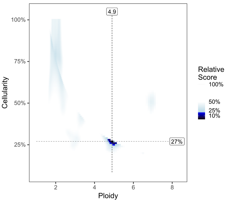
	Consider an Alternate solution	There seems to be a viable alternate solution around 75% / N=2 which may rescue this sample from failing otherwise. See instructions below to launch runs of purple with alternate cellularity/ploidy combinations.
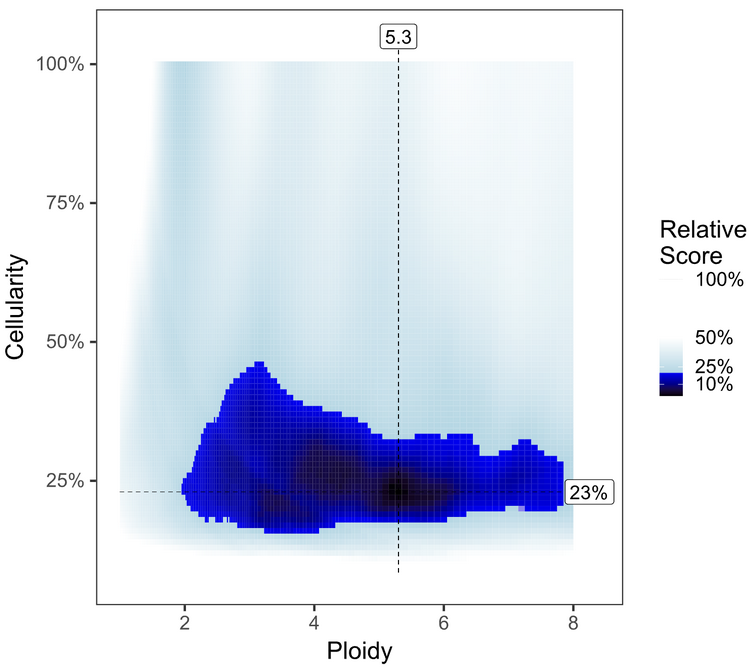
	Fail the Sample	While some solutions are above 30% cellularity, this nebulous cloud shape on a mostly blue background suggests the algorithm had trouble prioritizing solutions and the likely true solution is below 30%.

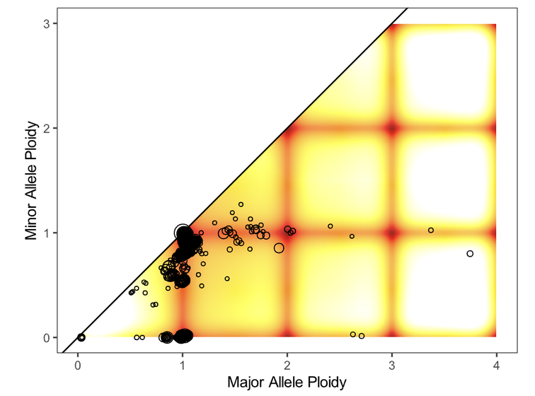
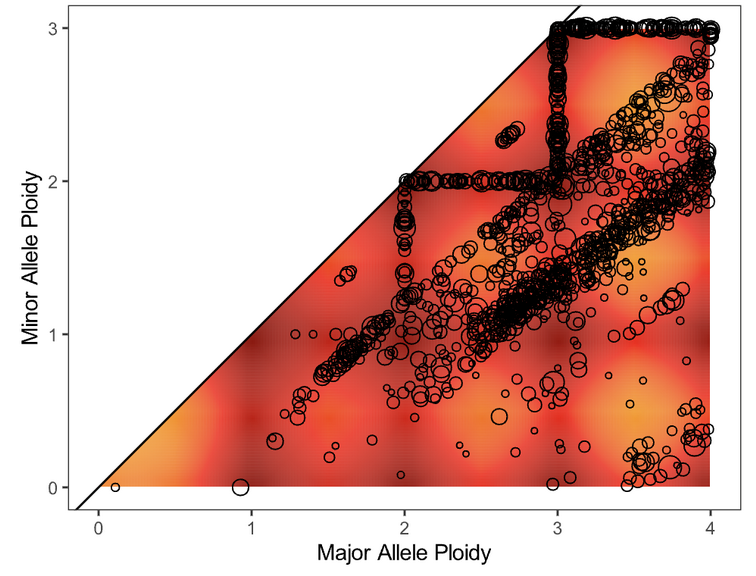
Next, evaluate the fit of the solution to the data by opening the file purple.segment_QC.png. The plot depicts the likelihood (as a penalty) of minor and major allele copy numbers based on the chosen cellularity/ploidy solution and the observed data. A heatmap showing which copy number regions have a high probability of containing segments, according to the predictive model generated, is overlaid by the observed segments (plotted as circles representing the size of the segment in number of supporting variants).

Preferred solutions have a close match between observation and prediction; that is, most segments occur in red/yellow regions (high probability), not white regions (low probability). It is ideal but not necessary for all segments to occur in high-probability regions of a solution.

Table 6 Evaluating the fit of the segments of a chosen cellularity/ploidy solution

Plot	Action	Guidance/Reasoning
	None	Fit looks good
	Consider an Alternate solution	Large distance between clusters of alleles will lead to an unlikely CNV track
	Fail the Sample	This sample appears to be hypersegmented. While this can occasionally be a biological phenomenon (like HRD), it is more likely that this sample is of low purity and that segments were not merged in PURPLE because breakends were missed since their structural variants were at low VAF. Check the mutations list in case the high segmentation can be explained by a DNA repair deficiency (eg. BRCA1 knockout).

Note the acceptable solution for recording in MISO later in Updating QCs.

Alternative PURPLE solutions

Interpreting the WGTS Report

Proceed with review of all informatics results using the HTML output. In this step, biomarker calls are manually reviewed in order to write the genome interpretation statement later.

Genomic Landscape

Note the percentile which the tumour mutation burden (TMB) is in, for the given tumour type. Refer to expected median TMB for the given tumour type in TCGA if it exists.

Evaluate actionable biomarkers for reporting: Oncokb reports TMB > 10 and MSI-H, and NCCN reports HR-D, as actionable.

• Large confidence intervals around the MSI score (spanning several result-interpretations, for example both MSI and MSS) are to be considered inconclusive. Inconclusive samples may be sent for PCR confirmatory testing.

• If HRD or MSI are positive, look for a somatic driver mutation: BRCA1, BRCA2, RAD51C, RAD51D, or PALB2 for HRD and MLH1, MSH2, MSH6, or PMS2 for MSI. If no mutations are reported within these genes, consider manually verifying filtered calls in IGV. There won’t always be one: the mutation may be germline or the phenotype may arise from methylation, among other explanations.

Always include a comment on MSI status, whether it is classified as MSI-High or Inconclusive. If the confidence interval spans multiple interpretations (e.g., overlaps both MSI and MSS thresholds), it should be explicitly described as inconclusive, and consideration should be given to PCR-based confirmatory testing.

SNVs and IN/DELs

SNVs and INDELs are reported according to the following filtering criteria:

Table 7 SNVs and InDels

Filter	Threshold
Variant Allele Frequency (VAF)	≥ 10% for SNVs and ≥ 20% INDELs
Supporting Reads	≥ 3 alt reads / ≥ 8 total reads; ≥ 4 reads in normal
OncoKB	All level 1-4, R variants which pass the above criteria All “Oncogenic”, “Likely Oncogenic” and “Predicted Oncogenic” alterations which pass the above criteria

Review all actionable and/or oncogenic mutations using Whizbam links for alignment artifacts. Whizbam links can be navigated from the data_mutations_extended_oncogenic.txt file.

Alterations which are deemed artifacts are to be removed from the data_mutations_extended.txt file and recorded into a new file labeled data_mutations_failed.txt. The data_mutations_extended.txt file has more than 100 columns and can be difficult to navigate; for convenience, the whizbam links for all mutations, and oncogenic mutations, are copied to whizbam_all.txt and whizbam_oncogenic.txt respectively.

Dinucleotide substitutions which are represented as two individual mutations are to be merged. Merged variants should be recorded in a new file named data_mutations_merged.txt. Copy both original individual annotations to this file, along with a third record of the final merged variant. To perform this merge, please follow this step-by-step procedure in the Merging and Annotating Mutations Representing the Same Event🔒 document on CGI:How-to wiki page.

Copy Number

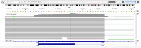
Review all Copy Number Variants by dragging the file purple.seg into your IGV browser. Evaluate each gene by inputting the name of that gene in the Location box of the browser.

Consider whether the segment, as outlined in the window labeled “purple”, includes the entire gene.

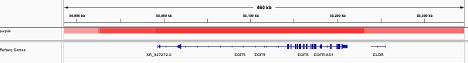
Above, the deep red section perfectly aligns with the gene EGFR in the Refseq window, supporting that the amplification indeed covers the entire gene.

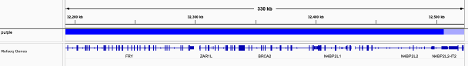
Deletions follow a similar logic: ensure the entire gene is bracketed by the deletion, as exemplified by the BRCA2 deletion in deep blue above.

If CNVs are partial, consult OncoKB or other relevant literature to explore whether partial deletions/amplifications are as oncogenic as full ones. If you find they are not, the CNV can be manually removed from the JSON.

Fusion and Structural Analysis

Review the fusions and/or structural variants in Whizbam.

The Whizbam links for fusion partners can be found in the file.

1. Open report/fusion_blurb_urls.tsv and copy the desired link into your browser to access the corresponding visualization.

2. Load the arriba/fusions.tsv file and review the following columns:

   • Confidence: Indicates the reliability of the predicted fusion.

   • Coverage: Describes the total number of reads supporting the fusion.

   • Number of split reads and discordant mates: Reflects the evidence for the fusion event.

   How to interpret Arriba results🔒.

3. In the Whizbam window, choose a read from one side of the fusion and click ‘View mate in split screen’. Ensure both mates map well by assessing for alignment artifacts such excessive numbers of mismatches or ambiguous mapping.

   • If the fusion is predicted by the arriba program, copy arriba’s fusions.pdf file into the MAVIS/ directory and check read support (coverage >=10X). Oncogenic fusions are generally highly expressed, as such a high coverage value is evidence of a true positive.

If an alignment looks like an artifact:

• Perform a BLAT analysis of the supporting reads to ensure alignments map non-ambiguously to this region. To do this, right click on the read and select ‘Blat read sequence’. This will perform a sensitive search for alternative alignments that the aligner did not report. Reads with multiple alignments are likely artifacts.

• Alterations which are deemed artifacts should be removed from the report/data_fusions_oncokb_annotated.txt file and the djerba_report.json and recorded into a new file labeled data_fusions_failed.txt.

Review Known Variants

If prior knowledge of previous sequencing results or biomarkers is known, review the relevant sections of the report to confirm and note abnormalities:

Table 8 Review known variants

Abnormality	Potential Cause	Action
Lack of expected alteration, or presence of a mutation where the mutation is expected or not expected	Lack of coverage for the expected mutation Sample swap Mutation is filtered	Verify coverage for the region by inspecting the bam file in Whizbam Whizbam links appear in the rightmost column of the data_mutations_extended_oncogenic.txt intermediate data file Check for sample swaps Confirm mutation was not removed by pipeline by reviewing the MuTect2 VCF file
Prior sequencing results are not confirmed	Low coverage for the expected mutation Sample swap Mutation is filtered	Verify coverage for the region by inspecting the bam file in Whizbam Check for sample swaps Confirm mutation was not removed by pipeline by reviewing the MuTect2 VCF file

If a discrepancy is noted, the sample should be marked as failed in MISO according to the QM-024. Quality Control and Calibration Procedures🔒 SOP. The report is to be regenerated with the FAIL flag as in Failed WGTS Report.

Updating QCs

Once everything is reviewed, follow the QC update procedure on QM-036. Quality Control Approval Procedure🔒:

1. Update the quality control field in MISO for “Purity”

2. Sign off on the “Informatics Review” in Dimsum.

Draft Report Generation

1. Generate an interpretation statement based on the findings from above. Include summaries of landscape, snv/indel, structural alterations, and copy number analysis. You can use blurbomatic to generate this statement. To run it, use:

   blurbomatic.py < ${REQUISITION_ID}_v1_report.json
   

Edit the generated interpretation statement if needed and save it under results_summary.txt in the report subdirectory of the working directory created in Set up a Djerba working directory. The interpretation statement may include simple HTML tags such as hyperlinks, bold/italic formatting, etc.

Note

⚠️ Blurbomatic is not yet configured to generate result summaries for the TAR assay or for failed reports of any assay type.

Use the following template as an example and refer to how to write a Genome Interpretive Statement🔒 for more details:

Table 9 Template for writing Genome Intrepretive Statement

Analysis Subsection	Example statement
Biological discrepancies	“The expected purity based on the pathologists’’ review is >80%, however, the inferred purity is below 40%. Variants are expected to have lower than expected VAFs”
Genomic landscape (step 3)	“This tumour has a TMB of xxx coding mutations per callable Mb which corresponds to the xxx percentile for $CANCER_TYPE. Genomic biomarker analysis returned no actionable biomarkers.”
SNV/Indel (step 4)	“Small mutation analysis uncovered loss of function mutations in xxx genes that suggest xxx.”
Fusions and structural alterations (step 5)	“Fusion analysis of RNA transcripts uncovered alteration of xxx genes that suggest xxx”
Integrated copy number and expression analysis (step 6)	“Integrated copy number and gene expression analysis uncovered alteration of xxx genes that suggest xxx”.
OncoKB treatment recommendations	Statements are taken from oncoKB: “Alteration xxx is a Level 1 mutation which the following treatment recommendations according to oncoKB”

2. Review and update report.json as necessary. For example, if a variant passes automated thresholds and appears in the report, but manual review determines it to be an artifact or not clinically significant, remove it manually from the JSON. Make any other required edits as well.

Note

To make the JSON easier to read and edit, open it in your IDE or run:

cat report.json | python3 -m json.tool > report_pretty.json

This will format the file for easier modification in a text editor.

3. Generate the JSON and PDF report with the interpretation changes and files.

Use the main djerba.py script in update mode, to generate revised JSON file:

$ djerba.py update -s report/results_summary.txt -j report/report.json -o report/

Use the main djerba.py script in render mode, to generate revised PDF file:

$ djerba.py render -j report/report.updated.json -o report/ -p

If necessary, the intermediate HTML file produced by Djerba may be also edited by hand. (This should only be done rarely, to resolve major formatting issues.) An HTML to PDF converter such as wkhtmltopdf may then be used to generate the PDF file. In this case, any subsequent edits by the clinical geneticist must be applied directly to the PDF, and not done with mini-Djerba.

Continue to Review the Draft Report ➡️

Example Djerba WGTS session

The following is an example sequence of commands used to generate a clinical report with Djerba. It is intended as a guide to CGI staff for report generation. The commands are for illustration only, not a fixed script to be followed. Comments are prefixed with #:

$ ssh ugehn.hpc
$ sudo -u svc.cgiprod -i
$ qrsh -P gsi -l h_vmem=16G
$ module load djerba
$ cd /.mounts/labs/CGI/cap-djerba/PASS01
$ mkdir -p PANX_1249/PASS01UHN-115
$ cd PANX_1249/PASS01UHN-115
$ mkdir report
$ djerba.py setup -a WGTS -p ../../PASS-01-config.ini --compact

# edit the config.ini file as detailed in the SOP
nano report/config.ini

# generate a draft report with Djerba; --verbose flag is optional, but gives helpful status updates
$ djerba.py --verbose report -i config.ini -o ./report

# review the HTML and edit the genomic_summary.txt file
$ nano report/results_summary.txt
$ djerba.py update -s report/results_summary.txt -j report/report.json -o report/ -p

Change Log

Github commit log